Category: Uncategorized

In statistics, Greek letters are commonly used to represent various parameters and constants. Here is an overview of some of the most frequently used Greek letters and their meanings:

Common Greek Letters in Statistics

1. 𝛼α (Alpha):
   • Significance Level: Used in hypothesis testing, it represents the probability of rejecting the null hypothesis when it is true (Type I error rate).
   • Cronbach’s Alpha: A measure of internal consistency or reliability of a psychometric instrument.
2. 𝛽β (Beta):
   • Regression Coefficient: Represents the slope of the regression line in simple linear regression.
   • Type II Error Rate: Represents the probability of failing to reject the null hypothesis when it is false.
   • Power of a Test: Often used in the context of statistical power, where 1−𝛽1−β is the power of the test.
3. 𝛾γ (Gamma):
   • Shape Parameter: In the gamma distribution, 𝛾γ can denote the shape parameter.
   • Gamma Function: Extends the factorial function to real and complex numbers.
4. 𝛿δ (Delta):
   • Difference or Change: Represents a change or difference in a variable.
   • Effect Size: In some contexts, it is used to denote the effect size.
5. 𝜖ϵ (Epsilon):
   • Error Term: Represents the error term in regression models.
6. 𝜂η (Eta):
   • Eta-Squared (𝜂2η2): A measure of effect size in the context of ANOVA, representing the proportion of variance explained by a factor.
7. 𝜆λ (Lambda):
   • Rate Parameter: In the Poisson and exponential distributions, it represents the rate parameter.
   • Eigenvalues: In linear algebra, used in principal component analysis and other multivariate techniques.
8. 𝜇μ (Mu):
   • Population Mean: Represents the mean of a population.
9. 𝜈ν (Nu):
   • Degrees of Freedom: Represents the degrees of freedom in various statistical tests, such as the 𝑡t-test and chi-square test.
10. 𝜋π (Pi):
    • Mathematical Constant: Approximately 3.14159, the ratio of the circumference of a circle to its diameter.
    • Proportion: Sometimes used to denote a proportion in a population.
11. 𝜌ρ (Rho):
    • Correlation Coefficient: Represents the population correlation coefficient.
12. 𝜎σ (Sigma):
    • Standard Deviation: Represents the standard deviation of a population.
    • Summation Operator: In some contexts, ΣΣ (capital sigma) represents the sum.
13. 𝜏τ (Tau):
    • Kendall’s Tau: A measure of correlation used with ordinal data.
14. 𝜙ϕ (Phi):
    • Golden Ratio: Approximately 1.618, often appears in nature and art.
    • Standard Normal Distribution: The standard normal distribution’s probability density function is sometimes denoted as 𝜙ϕ.
15. 𝜒χ (Chi):
    • Chi-Square Statistic: Used in chi-square tests for independence and goodness of fit.
16. 𝜔ω (Omega):
    • Sample Space: Represents the set of all possible outcomes in a probability experiment.

These Greek letters play a significant role in formulating statistical models, conducting hypothesis tests, and representing key statistical measures.

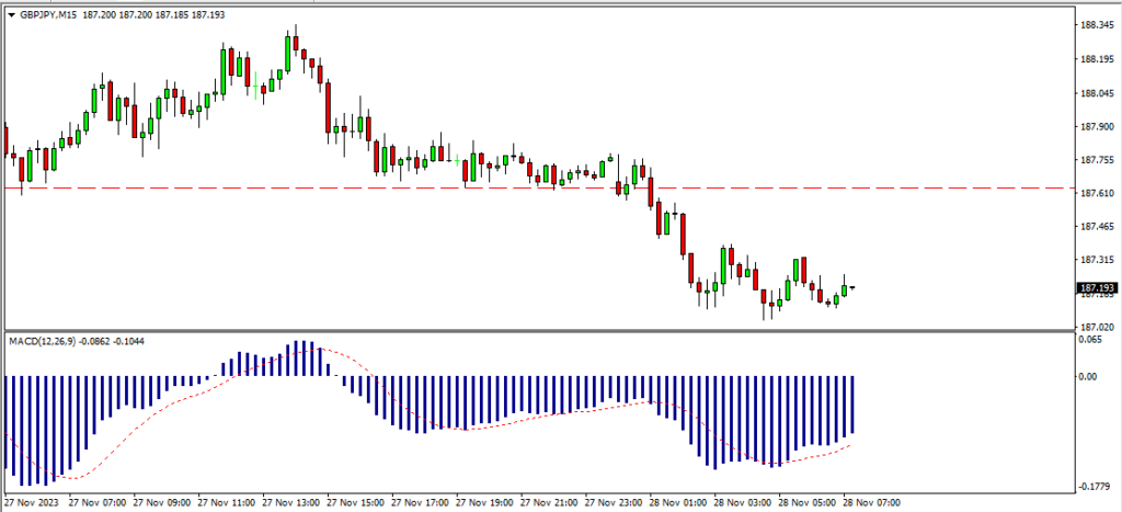
Early drop showing the signs of a bearish day. Or will it bounce back and try to break again?

Early drop showing bearish sign

Since we spotted a divergence on 4 hours the pair has dropped more than 100 pips. Call it a successful divergence or just a drop from strong rejection area, bears have been winning so far.

Since the opening today this pair has dropped more than 50 pips. We expect it to bounce back up near the 50 MA and drop again from there. There is a strong support near 186.382. It is now more likely that the pair will travel to that area and bounce back up from there.

So the mood remains bearish unless it truly breaks above 50, then we will look for a buy set up.

Detecting support and resistance levels in financial data involves analyzing historical price movements to identify levels at which the price has historically had difficulty moving below (support) or above (resistance). Here’s a basic example of how you can use Python and a popular library like pandas to detect support and resistance levels:

import pandas as pd
import matplotlib.pyplot as plt
import numpy as np
from scipy.signal import argrelextrema

# Load historical price data (you can get this data from a financial API or a CSV file)
# For the sake of example, let's create a simple price dataset
data = {
    'Date': pd.date_range(start='2023-01-01', end='2023-12-31'),
    'Close': [100, 110, 95, 120, 90, 115, 105, 125, 85, 130, 110, 140]
}

df = pd.DataFrame(data)
df.set_index('Date', inplace=True)

# Smooth the data using a moving average to identify significant peaks and troughs
window_size = 3
df['SMA'] = df['Close'].rolling(window=window_size).mean()

# Identify local minima (support levels) and maxima (resistance levels)
minima_idx = argrelextrema(df['SMA'].values, np.less, order=window_size)[0]
maxima_idx = argrelextrema(df['SMA'].values, np.greater, order=window_size)[0]

support_levels = df.iloc[minima_idx]['Close']
resistance_levels = df.iloc[maxima_idx]['Close']

# Plotting
plt.figure(figsize=(10, 6))
plt.plot(df.index, df['Close'], label='Close Price')
plt.plot(df.index, df['SMA'], label=f'SMA ({window_size} periods)')
plt.scatter(support_levels.index, support_levels.values, color='green', label='Support Levels', marker='^')
plt.scatter(resistance_levels.index, resistance_levels.values, color='red', label='Resistance Levels', marker='v')
plt.title('Support and Resistance Levels Detection')
plt.xlabel('Date')
plt.ylabel('Price')
plt.legend()
plt.show()

In this example:

• We use a simple moving average (SMA) to smooth the price data.
• We identify local minima and maxima in the smoothed data using argrelextrema from scipy.signal.
• The identified minima correspond to potential support levels, and the identified maxima correspond to potential resistance levels.
• We plot the original closing prices along with the smoothed curve and mark the detected support and resistance levels.

This is a basic example, and in a real-world scenario, you might want to use more sophisticated techniques and additional indicators to improve the accuracy of support and resistance level detection. Additionally, you could explore libraries like ta-lib for technical analysis or machine learning models for more advanced pattern recognition.